5.1.4. Current loop tuning

This section provides guidance on the following aspects of tuning the current loop in FOC:

• What constitutes a well-tuned current controller?
• How do I adjust the current control loop gains in MCAF?
• How can I use autotuning in the Tune page of motorBench^® Development Suite to make gain tuning easier?
• Are the default current control loop tuning criteria in motorBench^® Development Suite good enough to meet the requirements of most systems?

5.1.4.1. Background

As mentioned in the FOC component section on current control, MCAF uses a pair of PI controllers with saturation and antiwindup. The PI control gains are proportional gain \(k_{ip}\) and integral gain \(k_{ii}\).

Current loop tuning in FOC can be a challenging task, for a number of related reasons:

• Control variables of interest (d-axis and q-axis currents) are not directly measurable with test equipment, and exist only as software variables within the microcontroller
• Aside from directly assessing step responses of dq-frame currents, evaluating control performance is an unclear task
• Control problems are not readily apparent
  • a motor may be rotating very smoothly but still exhibiting poor current control behavior
  • observable effects are usually audible but are unclear indicators such as clicks, clunks, chatter, hiss, or screeching
  • sinusoidal distortion when measuring phase currents may be viewed as a disproportionate concern
• FOC is a 2 × 2 MIMO control system with some subtleties (inductive cross-coupling and saturation behavior for all PMSM, with anisotropic behavior for motors with rotor saliency or fast mechanical time constants)

The good news is that tuning a current controller with FOC is usually forgiving and does not have to be optimal, and the control gains calculated in motorBench^® Development Suite are usually acceptable and conservative.

5.1.4.2. Evaluating control performance

Several goals of the current controller are listed below:

• Reference tracking — make the measured current follow the current reference input with zero steady-state error.

  • Torque generated by the motor is proportional to the Q-axis current \(I_q\), so controlling \(I_q\) controls the torque.
  • D-axis current \(I_d\) modulates the airgap flux. For SPM motors, the torque per ampere is maximized by \(I_d = 0\), but for IPM motors, a nonzero value of \(I_d < 0\) can be used to increase efficiency, as calculated by the MTPA equations. Any PMSM can also utilize \(I_d < 0\) to counteract part of the back-emf and extend the operating velocity range, when required, through flux weakening.

  An important quantity for reference tracking is the control bandwidth, along with time-domain metrics such as rise time and settling time, shown in Figure 5.14.

• Overshoot management — we don’t want undesirable transient behavior following a step change in reference current; we want it to settle quickly and avoid reaching excessive values. Overshoot can be described quantitatively as a normalized fraction; for example, if a reference current step from -1 A to 1 A (a change of 2 A) leads to a maximum current during the transient of 1.3A, then the overshoot is equal to \((1.3 - 1)/(1 - (-1)) = 0.15\).

  An example of overshoot is shown in Figure 5.14.

  

  Figure 5.14 Example of time-domain metrics for the step response of the mildly interesting transfer function \(H(s) = \dfrac{-400s+40000}{s^4+11s^3+720s^2+5200s+40000}\). Rise time measures the time needed to transition from 10% of the step change to 90% of the step change. Settling time measures the time until the step response stays within a given bound, here ±5%.

• Disturbance rejection — noise, back-emf harmonics, and dead-time distortion are effects that perturb the motor current. A well-tuned current control loop will keep the current error small. Disturbance rejection can be characterized quantitatively by a stiffness transfer function \(H(s) = \partial V/\partial I\) that represents the voltage disturbance required to make a particular change in current. [1] In closed loop at frequencies much lower than the current loop bandwidth, this stiffness can be very large, but in open loop and at high frequencies it is the per-phase impedance \((R+j\omega_e L)\) of the stator.

• Stability — we want oscillations in current to decay and not persist or grow. An important quantity for stability is phase margin \(\phi_m\).

More specifically, the tuning goals are to constrain error, constrain overshoot, and maximize bandwidth:

• Current control error can cause vibration and audible noise within the motor. In extreme cases it can add excess thermal dissipation, damage components (if the overcurrent is not detected), or cause nuisance faults (if the overcurrent is detected).

• Phase margin should be selected to keep overshoot small. Acceptable values of overshoot are typically in the 0-10% range. This depends on the application as well as the frequency content of the current reference. The worst-case step of full negative current to full positive current is not necessarily something that occurs in a real application, but if it is, causing false overcurrent faults should be avoided. For example, a motor drive that can accept reference currents up to 10 A that undergoes a worst-case step from -10 A to +10 A and has a 10% overshoot would reach a maximum current of +12 A. There should be enough design margin between this maximum current and the minimum overcurrent threshold to allow room for noise while still avoiding false overcurrent faults.

• Current control bandwidth should generally be maximized as long as it does not degrade stability or introduce excessive noise into the motor current. Typical 3dB current bandwidth of industrial motor drives are 5-15% of the PWM frequency, or 1-3 kHz for a 20 kHz PWM. This is desirable even if the overall motor control bandwidth of position or velocity is slow, for example a pump or fan operating at constant velocity. It improves disturbance rejection and reduces the duration of overcurrent events.

  Applications that do require fast acceleration (robotics and e-mobility, for example) are constrained by the performance of the current loop; the velocity loop bandwidth is generally 5-10 times lower than the current loop bandwidth.

5.1.4.3. Examples of poorly-tuned and well-tuned current loops

The best way to evaluate current loop performance is with a step response test at constant velocity. The easiest way of doing this with MCAF is to use the square-wave perturbation of the test harness (see Square wave velocity command disturbances to a velocity controller with fixed velocity command) with one of the following:

• clamping the rotor to prevent movement
• running the motor with open-loop commutation, using a fixed commutation angle (see section on commutation issues)
• controlling the motor to run at constant velocity, with a low-bandwidth velocity loop. (This lets the motor accelerate or decelerate slightly; rotor inertia will smooth out velocity.)

A square wave perturbation in the 20 Hz - 200 Hz range is recommended: for 20 kHz control rate, this corresponds to values of motor.testing.sqwave.halfPeriod between 500 and 50. In general the period of the square wave should be just long enough for transients to complete.

Note: Pay special attention to motor commutation. Sensorless position estimators add their own sources of error to commutation angle, and may not be practical to use at zero speed to test current loop tuning. Except where noted, all graphs in this section show data from a motor using a quadrature encoder for commutation. See the last section on commutation issues for more information.

Operation with open-loop commutation may also be required for current loop tuning if the normal MCAF startup sequence fails to run or transition properly into closed-loop commutation.

5.1.4.3.1. Current loop tuning at zero velocity

Figure 5.15 shows an example of the current loop step response of the Nidec Hurst DMA0204024B101 motor operated with MCAF on the dsPICDEM^® MCLV‑2 Development Board, with default tuning in motorBench^® Development Suite.

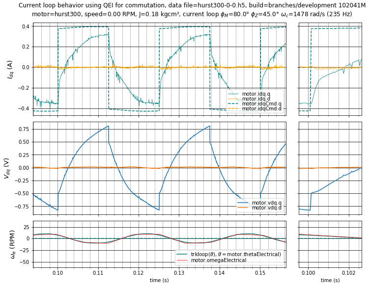
Figure 5.15 Case 0: Current loop step response with phase margin \(\phi_m = 80^\circ\) and PI phase lag at crossover \(\phi_z = 45^\circ\) (\(K_p =\) 0.414 V/A, \(K_i =\) 613 V/As). All cases in this section have dead time reduced from 2 μs to 1.2 μs to minimize the effects of dead-time distortion. Step-response graphs included in this section all contain values for phase margin, PI phase lag at crossover (see section on performance criteria for a definition), and crossover frequency \(\omega_c\) in the graph title.

This current loop has a low bandwidth — so low that current does not reach its steady-state value because the velocity is allowed to vary, and the changing back-emf, which results from changes in velocity, acts as a disturbance to the current loop. To avoid this effect, the product of mechanical time constant \(\tau_{m1} = \frac{2JR_s}{3K_e{}^2}\) and current loop bandwidth should be much greater than 1. For the Nidec Hurst DMA0204024B101, the mechanical time constant \(\tau_{m1} =\) 3.25 ms, and in this particular instance (Case 0) the product \(\omega_c\tau_{m1}\) = 4.8, not high enough to mitigate the effect of changing back-emf.

Several other cases, with the same motor and board, are summarized in Table 5.1.

Table 5.1 Tuning parameters for six different cases.

case	\(\phi_m\)	\(\phi_z\)	\(\omega_c\) (rad/s)	\(f_c\) (Hz)	\(K_p\) (V/A)	\(K_i\) (V/As)
0	80.0°	45.0°	1478	235	0.414	613
1	70.0°	25.0°	3709	590	1.226	2121
2	45.0°	12.0°	12759	2031	4.487	12168
3	30.0°	5.0°	19662	3129	7.038	12107
4	55.0°	3.0°	12458	1983	4.473	2920
5	80.0°	45.0°	1355	216	0.418	566

The next case (1), shown in Figure 5.16, has slightly lower phase margin and PI phase at crossover, which results in higher bandwidth and a better step response. This looks similar to Case 0 in shape, but the time scale here is 2.5× faster.

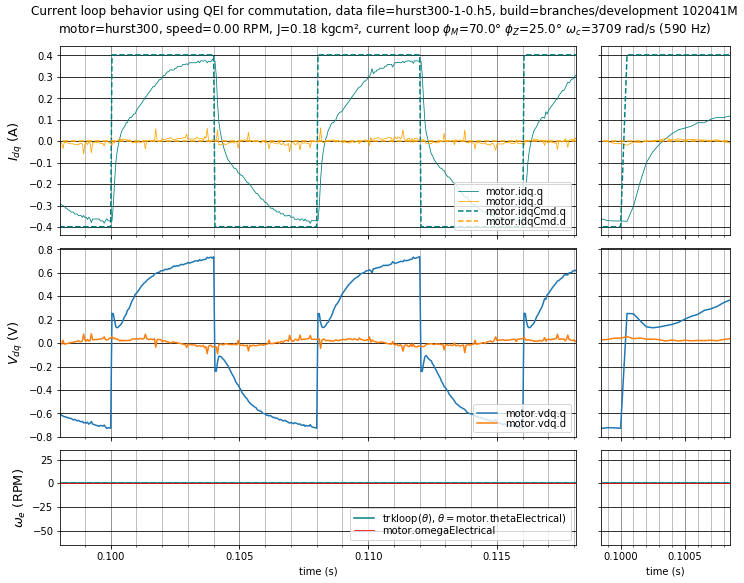
Figure 5.16 Case 1: Current loop step response with \(\phi_m = 70^\circ,\;\phi_z = 25^\circ\) (\(K_p =\) 1.226 V/A, \(K_i =\) 2121 V/As).

The early part of the step response (during the first 100 μs or so) is dominated by the proportional gain \(K_p\). This causes a rapid pulse in voltage. As the current approaches its reference value and the error decreases, the response becomes dominated by the integral term; the integral gain \(K_i\) determines how fast this transition occurs.

The response of Case 1 can still be improved.

Case 2, in Figure 5.17, shows a well-tuned current loop. This has fast bandwidth of about \(f_s/10\) (where \(f_s\) is the sampling and control rate) and a reasonably good step response without overshoot. Improving bandwidth beyond \(f_s/10\) can be done, but is tricky and requires careful attention to discrete-time design as well as the sample-to-output delay.

Again, note the initial voltage impulse beyond the final value required to maintain current at its reference value.

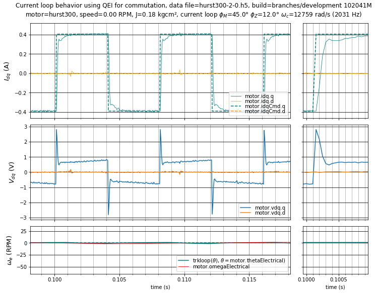
Figure 5.17 Case 2: Well-tuned current loop step response with \(\phi_m = 45^\circ,\;\phi_z = 12^\circ\) (\(K_p =\) 4.487 V/A, \(K_i =\) 12168 V/As).

Case 3, in Figure 5.18, shows a current loop with gains that are too high, causing excessive overshoot. Here the overshoot is only about 12%, but if we operate at nonzero velocities the overshoot will get worse.

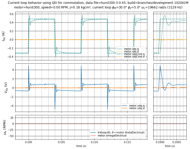
Figure 5.18 Case 3: High-gain current loop step response with \(\phi_m = 30^\circ,\;\phi_z = 5^\circ\) (\(K_p =\) 7.038 V/A, \(K_i =\) 12107 V/As).

Case 4, in Figure 5.19, shows a current loop with about the same proportional gain \(K_p\) but a much lower integral gain. The proportional gain yields a very good short-term response, but the low integral gain causes a much slower settling time towards the final value.

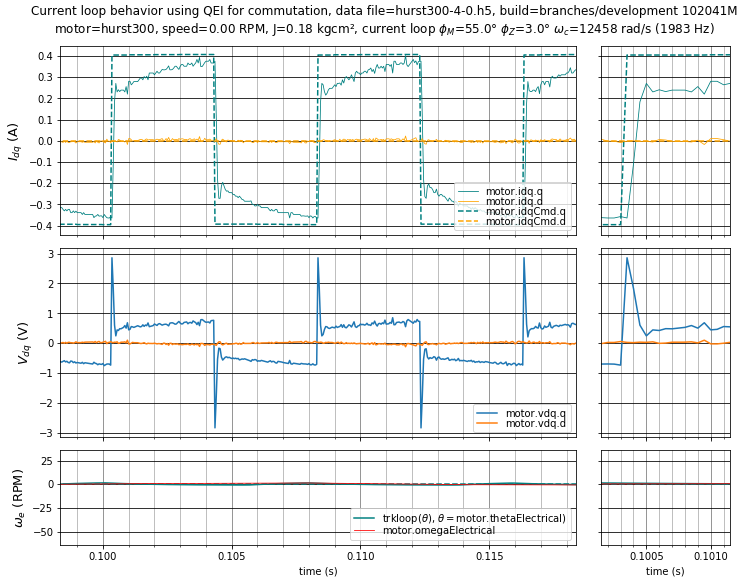
Figure 5.19 Case 4: Current loop step response with \(\phi_m = 55^\circ,\;\phi_z = 3^\circ\) (\(K_p =\) 4.473 V/A, \(K_i =\) 2920 V/As).

Finally, Case 5, in Figure 5.20, shows the same phase margin and PI phase lag at crossover as Case 0, but with an external inertial load added to increase the rotor inertia by about a factor of 3. Current loop tuning doesn’t change much, but note the improved settling of the current loop caused by the reduction in velocity fluctuation.

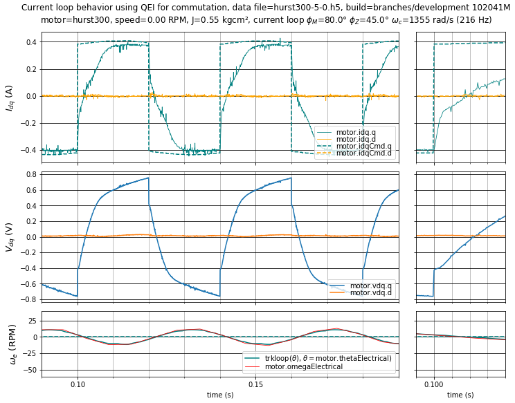
Figure 5.20 Case 5: Current loop step response with \(\phi_m = 80^\circ,\;\phi_z = 45^\circ\) but with \(J \approx 3J_0\) (\(K_p =\) 0.418 V/A, \(K_i =\) 566 V/As)

5.1.4.3.2. Current loop tuning at nonzero velocity

At low velocities, the current loop step response does not change much.

As the rotor velocity increases, there are cross-axis coupling effects between the d- and q-axes that change the step response somewhat. [2] For this reason, it is important to verify current loop tuning at the upper end of the velocity range. Avoiding voltage saturation is important for the purposes of tuning, so either use an elevated DC link voltage, or choose a velocity that is about 80-90% of maximum velocity.

Below are the step responses of cases 1-3 at 1200 RPM and 2400 RPM.

In the low-gain controller cases of Figure 5.21 and Figure 5.22, the voltage disturbances of dead-time distortion and back-emf harmonics can cause moderate error, compared to the step response seen at zero velocity.

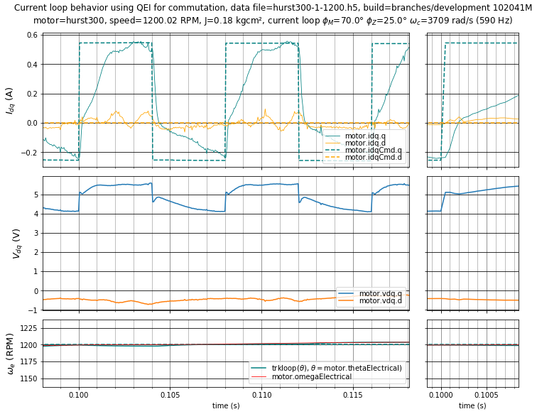
Figure 5.21 Case 1: Current loop step response of low-gain controller with \(\phi_m = 70^\circ,\;\phi_z = 25^\circ\) (\(K_p =\) 1.226 V/A, \(K_i =\) 2121 V/As) at 1200 RPM.

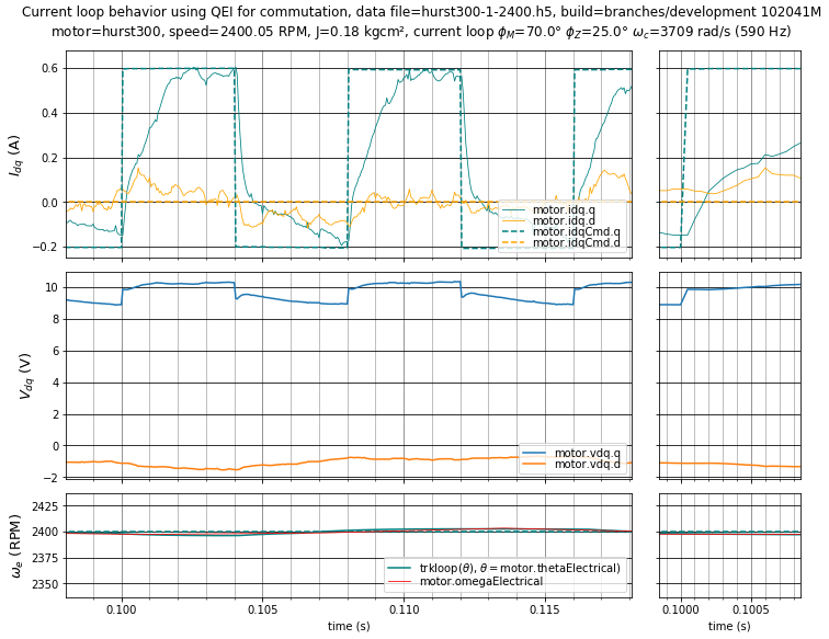
Figure 5.22 Case 1: Current loop step response of low-gain controller with \(\phi_m = 70^\circ,\;\phi_z = 25^\circ\) (\(K_p =\) 1.226 V/A, \(K_i =\) 2121 V/As) at 2400 RPM.

In the well-tuned case of Figure 5.23 and Figure 5.24, the increased gain improves disturbance rejection, reducing the error from the current reference.

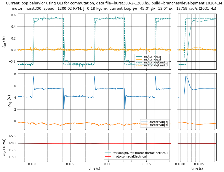
Figure 5.23 Case 2: Well-tuned current loop step response with \(\phi_m = 45^\circ,\;\phi_z = 12^\circ\) (\(K_p =\) 4.487 V/A, \(K_i =\) 12168 V/As) at 1200 RPM.

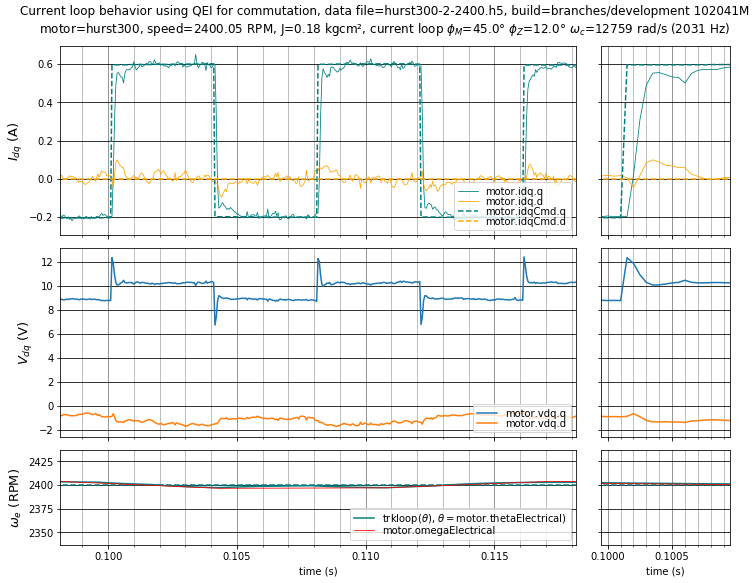
Figure 5.24 Case 2: Well-tuned current loop step response with \(\phi_m = 45^\circ,\;\phi_z = 12^\circ\) (\(K_p =\) 4.487 V/A, \(K_i =\) 12168 V/As) at 2400 RPM.

In the high-gain case of Figure 5.25 and Figure 5.26, the current overshoot increases with increasing velocity, reaching 20% overshoot at 2400 RPM. This is undesirable and may become worse than shown here due to several causes:

• part-to-part variations in the motor parameters
• part-to-part variations in current sense circuitry in the drive electronics
• resistance and back-emf changes with temperature
• inductance changes with iron saturation

In short: if at all possible, avoid overshoot and leave design margin for parameter tolerances.

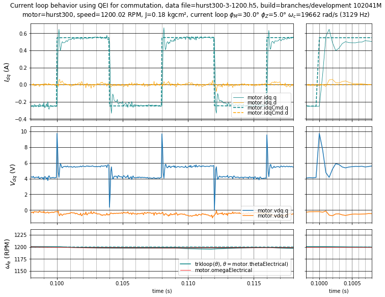
Figure 5.25 Case 3: High-gain current loop step response with \(\phi_m = 30^\circ,\;\phi_z = 5^\circ\) (\(K_p =\) 7.038 V/A, \(K_i =\) 12107 V/As) at 1200 RPM.

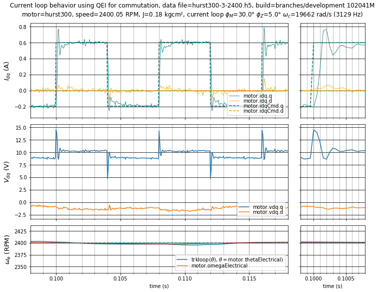
Figure 5.26 Case 3: High-gain current loop step response with \(\phi_m = 30^\circ,\;\phi_z = 5^\circ\) (\(K_p =\) 7.038 V/A, \(K_i =\) 12107 V/As) at 2400 RPM.

5.1.4.3.3. Effects of sample-to-update delay

A critical bottleneck in providing stable high-bandwidth current loops is the sample-to-update delay \(T_{su}\). This is the delay between the instant the ADC inputs are sampled, and the instant the duty cycle of the transistors changes based on the values of those sampled inputs.

Reducing the delay \(T_{su}\) allows for a more stable current loop at a given bandwidth, or a higher bandwidth for equivalent stability. The difference is most pronounced at high bandwidths (5% or more of the sampling frequency, e.g. 1 kHz and greater for a 20 kHz sampling-and-update rate)

MCAF R6 recommends the use of double-update PWM to help reduce sample-to-update delay.

5.1.4.4. Tuning criteria and motorBench^® Development Suite

5.1.4.4.1. Performance criteria definitions

The autotuning feature of motorBench^® Development Suite allows adjustment of two performance criteria for both the current and velocity loops:

• Phase margin \(\phi_m\) is the difference between -180° and the phase of open-loop gain transfer function at the crossover frequency \(\omega_c\), where the open-loop gain has magnitude 1. This represents design margin from the point of instability. Decreased phase margin generally raises both proportional gain \(K_p\) and integral gain \(K_i\). This can increase the maximum achievable bandwidth and improve the performance of reference tracking and disturbance rejection, but at the cost of decreased stability.
• PI phase lag at crossover \(\phi_z = \tan^{-1} K_i/K_p\omega_c\) is the phase lag of the PI controller at the crossover frequency. Decreased PI phase lag at crossover decreases the corner frequency (or “zero”) of the PI controller, decreasing integral gain \(K_i\) and increasing proportional gain \(K_p\). With a fixed phase margin, this generally increases the current loop bandwidth, but at the cost of decreased gain at low frequencies, which reduces the controller’s disturbance rejection.

While phase margin may be familiar to engineers with a rudimentary knowledge of control systems, PI phase lag at crossover may not. Figure 5.27 shows a Bode plot of the current loop transfer functions for the Nidec Hurst DMA0204024B101, with the following elements:

• The plant transfer function G(s), representing voltage-to-current gain, is drawn in a thin dash-dot line
• PI controller transfer functions K(s), representing current-to-voltage gain, are drawn in dashed lines
• Open-loop gain transfer functions G(s)K(s) are drawn in solid lines
• The transfer functions are evaluated and marked with a small dot at the crossover frequency. Note that in Figure 5.27, the open-loop gain transfer function has a phase of -105°, in order to meet the phase margin constraint of 75°.
• The PI controller zero, which is the frequency where proportional and integral gain are equal and the phase is -45°, is marked with an open circle. The ratio of the PI controller zero to the crossover frequency is \(\tan \phi_z\), so that low values of PI phase lag at crossover push the controller zero to very low frequencies.

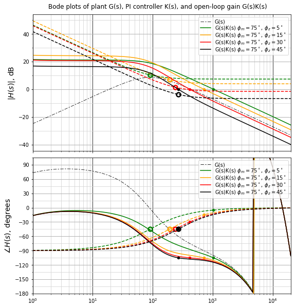
Figure 5.27 Bode plot of selected PI phase lags at crossover, with a phase margin of 75°.

5.1.4.4.2. Bode plots of example cases

Figure 5.28 shows a Bode plot of the examples for cases 0 - 4 discussed earlier in this section.

Cases 2 (\(\phi_m = 45^\circ,\;\phi_z = 12^\circ\)) and 3 (\(\phi_m = 30^\circ,\;\phi_z = 5^\circ\)) have the highest low-frequency open-loop gain, but the the lower phase margin of case 3 renders it undesirable.

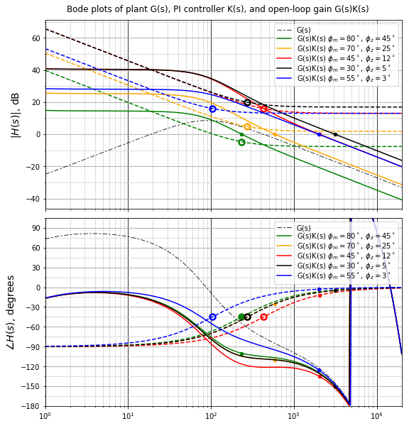
Figure 5.28 Bode plot of current loop transfer functions for example cases discussed in this section

5.1.4.4.3. Default values of performance criteria

The default values chosen for the current loop in motorBench^® Development Suite versions 1.15 – 2.35, namely \(\phi_m = 80^\circ,\;\phi_z = 45^\circ\), are stable for a very wide range of motors. They are also extremely conservative, and result in a current loop bandwidth that is rather low.

Microchip staff is re-evaluating these default values for a higher-performance recommendation. In the interim, if careful step-response testing is possible, consider reducing phase margin to the 50° – 70° range and reducing PI phase lag at crossover to the 8° – 20° range. Do not decrease these values below the defaults without testing. PI phase lags below 5° are not recommended without careful study.

Autotuning uses these performance criteria, rather than PI gains or loop bandwidth, as a normalized specification that is somewhat applicable across a wide range of motor and drive combinations. Are the exact values for phase margin and PI phase lag at crossover for the Nidec Hurst DMA0204024B101 shown here in the well-tuned case (\(\phi_m = 45^\circ,\;\phi_z = 12^\circ\)) applicable to all motors? No. Each motor and drive combination has different characteristics, and there are often subtle second-order effects that may warrant higher or lower settings.

If you have a motor that seems difficult to tune, please bring it to the attention of Microchip staff so that we can improve our recommendations.

5.1.4.5. Adjusting current control gains in MCAF

The best way to adjust current control gains in MCAF is to change the performance criteria (phase margin \(\phi_m\) and PI phase lag at crossover \(\phi_z\)) in the Tune page of motorBench^® Development Suite. This may require repeated iterations of code generation, however.

To fine-tune the current loop more quickly, it is possible to change the current loop gains at runtime directly, by changing the proportional and integral gains of both d-axis and q-axis current loops, using a real-time diagnostic tool to adjust the MCAF variables shown in Listing 5.1.

Listing 5.1

motor.idCtrl.kp
motor.idCtrl.ki
motor.iqCtrl.kp
motor.iqCtrl.ki

(Note that there are also runtime shift counts with the same variable names as the gains, preceded by an n, for example motor.idCtrl.nkp for the shift count corresponding to .kp. If the desired gain would overflow (above 32767 counts), then subtract one from the shift count and divide the gain counts by two. .kp = 38000, .nkp = 15, which is not representable, is equivalent to .kp = 19000, .nkp = 14, which is representable.)

The recommended approach is as follows:

• Make a copy of the initial gains generated by motorBench^® Development Suite, found in foc_params.h
• Adjust current loop gains at runtime, using a real-time diagnostic tool to perform step-response testing. The most important software variables to watch are
  • motor.idq.q — Q-axis current
  • motor.idqCmd.q — Q-axis current reference
  • motor.vdq.q — Q-axis voltage output from PI controller
• Determine desired software gains empirically
• Compute real-world gains corresponding to the software gains
• Adjust \(\phi_m\) and \(\phi_z\) in the Tune page of motorBench^® Development Suite to produce gains that are close to the desired real-world gains. (At this time, entry of PI gains in the Tune page is not possible, but it may be considered in future versions.)

5.1.4.5.1. Example

Listing 5.2 shows an example set of gains in foc_params.h generated by motorBench^® Development Suite.

Listing 5.2 foc_params.h

//************** PI Coefficients **************
//// Current loop
// phase margin = 80 deg
// PI phase at crossover = 45.000 deg
// crossover frequency = 1.478 k rad/s (235.238 Hz)
/* Current loop proportional gain */
#define KIP                                  2263      // Q15(  0.06906) = +414.36768 mV/A        = +414.42006 mV/A        - 0.0126%
#define KIP_Q                                  15
/* Current loop integral gain */
#define KII                                   167      // Q15(  0.00510) = +611.57227 V/A/s       = +612.53173 V/A/s       - 0.1566%
#define KII_Q                                  15

Suppose that a well-tuned current loop response can be obtained using a real-time diagnostic tool with the following software gains:

• motor.idCtrl.kp = motor.iqCtrl.kp = 24500
• motor.idCtrl.ki = motor.iqCtrl.ki =  3300

The engineering units can be computed by adjusting the original gain in engineering units by the ratio of new to old software values:

• \(K_p\) = (24500/2263) × 0.41437 = 4.4861 V/A
• \(K_i\) = (3300/167) × 611.57 = 12085 V/As

Then adjust phase margin \(\phi_m\) and PI phase lag at crossover \(\phi_z\) of the current loop in the Tune page of motorBench^® Development Suite to get close to these values. (Again, decreasing phase margin should increase both \(K_p\) and \(K_i\); decreasing PI phase lag at crossover increases \(K_p\) and decreases \(K_i\).)

5.1.4.6. Commutation angle issues during current loop tuning

Commutation angle accuracy is not particularly critical during current loop tuning, as long as the total error is manageable. Typically a commutation angle error of 15° electrical is acceptable for field-oriented control. High-frequency content (oscillation in the commutation angle) will show up as a disturbance orthogonal to the current vector; in the normal case where D-axis current is approximately zero and the current vector is primarily along the Q-axis, then the D-axis current will show oscillations from commutation angle errors, whereas similar oscillations in the Q-axis current will be much smaller.

If possible, perform step-response tuning using a quadrature encoder for commutation. Use a tracking loop time constant that is relatively slow: 5 ms is a good default choice.

If a quadrature encoder is not available, then operation at zero speed may not be possible with closed-loop commutation. (The AN1292 PLL estimator is generally stable at zero speed, but cannot provide useful torque, whereas the ATPLL has stability issues around zero speed.) If this is the case, use open-loop commutation instead, by taking the following steps using the test harness and a real-time diagnostic tool:

• turn on the commutation override
• use a fixed commutation angle by setting motor.testing.overrideOmegaElectrical = 0, which controls the commutation frequency.

At zero speed, mechanically clamping the rotor can be helpful, but is not necessary, and will not suppress small high-frequency vibrations.

Operation at nonzero speed to check current loop tuning should be done with closed-loop commutation. Again, a quadrature encoder is recommended, but a sensorless estimator may be used for commutation as long as the velocity is large enough for good performance.

5.1.4.6.1. Example using the AN1292 PLL

Similar current loop evaluation can be done using the AN1292 PLL at zero speed in closed-loop commutation. Figure 5.29, Figure 5.30, and Figure 5.31 show current loop evaluation of the Nidec Hurst DMA0204024B101 motor with the well-tuned current loop gains (\(\phi_m = 45^\circ,\;\phi_z = 12^\circ\)) that were used earlier in this section. To keep the current reference from changing quickly, the velocity loop bandwidth was lowered to around 2.2 Hz from the default tuning, by choosing \(\phi_m = 70^\circ,\;\phi_z = 20^\circ\). (This is not necessary in general — it just makes current loop tuning easier to avoid unnecessary distractions, and a higher-bandwidth velocity loop can be used after current loop tuning is complete.)

Steps in the current reference at 1 ms intervals are visible due to angle and velocity uncertainty from the estimator, but otherwise the current loop tuning behaves almost identically to the case where a quadrature encoder is used for commutation angle.

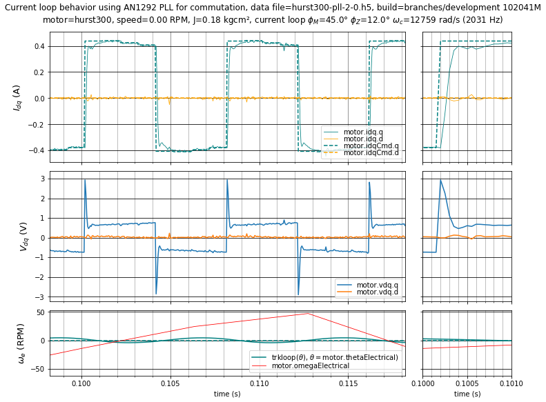
Figure 5.29 Case 2 with PLL: Well-tuned current loop step response with \(\phi_m = 45^\circ,\;\phi_z = 12^\circ\) (\(K_p =\) 4.487 V/A, \(K_i =\) 12168 V/As) at 0 RPM. Velocity tuning has \(\phi_m = 70^\circ,\;\phi_z = 20^\circ\).

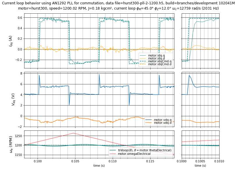
Figure 5.30 Case 2 with PLL: Well-tuned current loop step response with \(\phi_m = 45^\circ,\;\phi_z = 12^\circ\) (\(K_p =\) 4.487 V/A, \(K_i =\) 12168 V/As) at 1200 RPM. Velocity tuning has \(\phi_m = 70^\circ,\;\phi_z = 20^\circ\).

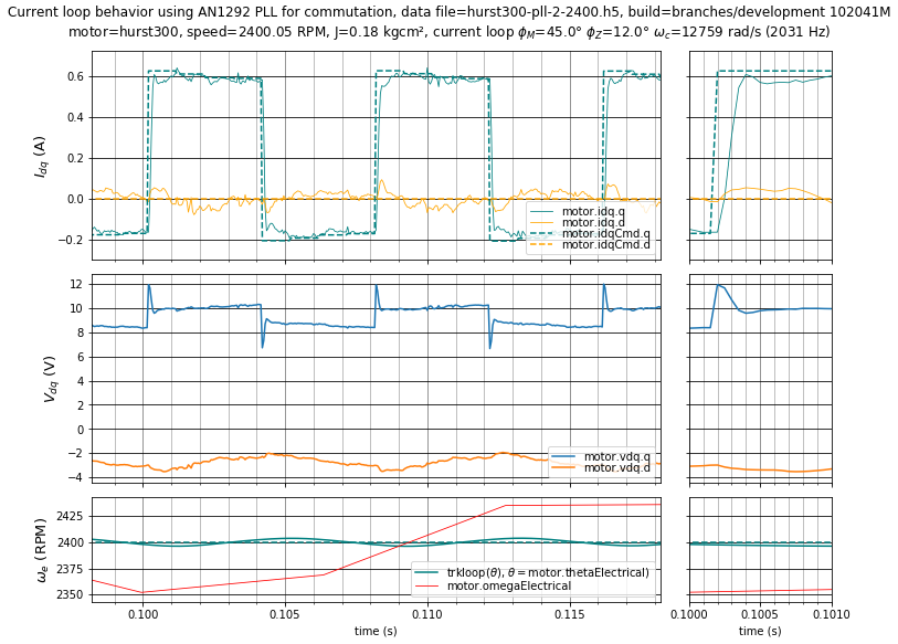
Figure 5.31 Case 2 with PLL: Well-tuned current loop step response with \(\phi_m = 45^\circ,\;\phi_z = 12^\circ\) (\(K_p =\) 4.487 V/A, \(K_i =\) 12168 V/As) at 2400 RPM. Velocity tuning has \(\phi_m = 70^\circ,\;\phi_z = 20^\circ\).

5.1.4.7. References

[1]	F. B. del Blanco, M. W. Degner and R. D. Lorenz, “Dynamic analysis of current regulators for AC motors using complex vectors”, IEEE Transactions on Industry Applications, vol. 35, no. 6, pp. 1424-1432, Nov/Dec. 1999.

[2]	F. Briz, M. W. Degner and R. D. Lorenz, “Analysis and design of current regulators using complex vectors”, IEEE Transactions on Industry Applications, vol. 36, no. 3, pp. 817-825, May/June 2000.