5.4.1. Flux weakening
5.4.1.1. Motivation
Many applications require the motor to be run at a velocity greater than the rated velocity of the motor. In a PMSM, the back emf increases in proportion to the rotor velocity. Steady-state stator voltage equations for a typical PMSM are given by 5.37. Here, \(R_{s}\) is per-phase stator resistance, \(L_{d}\) and \(L_{q}\) are motor inductance values in the d and the q axes, respectively, while \(V_{ds}\) and \(V_{qs}\) are stator voltage components in the d and the q axes, respectively. Back emf \(E_{Mag}\) lies in the q axis and is given by 5.38. Here, \(\omega_e\) is the rotor velocity in electrical rad/s and \(\Psi_{PM}\) is the back emf constant in volts per electrical rad/s.
5.37 shows that the q-axis stator voltage will increase as the back emf increases. This is depicted in Figure 5.57. At around the rated motor velocity, the voltage reaches the motor’s rated voltage value and it cannot be increased further. Often, this rated voltage also corresponds to the maximum possible voltage that can be obtained from the inverter due to DC link voltage limitations.
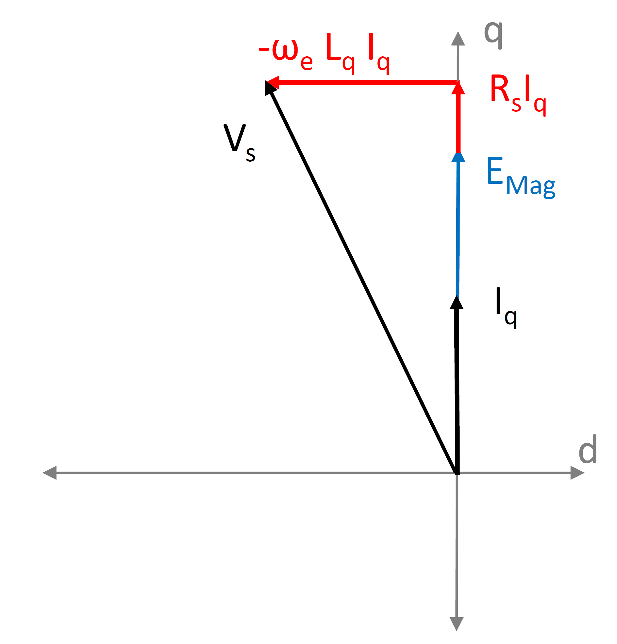
Figure 5.57 PMSM vector diagram: \(I_{d} = 0\)
In order to allow a further increase in motor velocity, it is necessary to restrict the increase in \(V_{qs}\) while allowing \(E_{Mag}\) to increase. For a positive velocity, this is achieved by making the \(\omega_e L_{d} I_{d}\) term negative, which in turn is done by making \(I_{d}\) negative. Figure 5.58 shows the vector diagram with a negative \(I_{d}\) injected in the motor. Here, \(V_{s}\) (dashed black arrow) shows the stator voltage vector with \(I_{d} = 0\), whereas \(V_{s\_fw}\) (solid black arrow) shows the stator voltage vector with \(I_{d} < 0\). Due to the opposing effect of the negative \(\omega_e L_{d} I_{d}\) term, the magnitude of \(V_{s\_fw}\) is lower than the magnitude of \(V_{s}\), for the same values of \(E_{Mag}\) and \(I_{q}\).
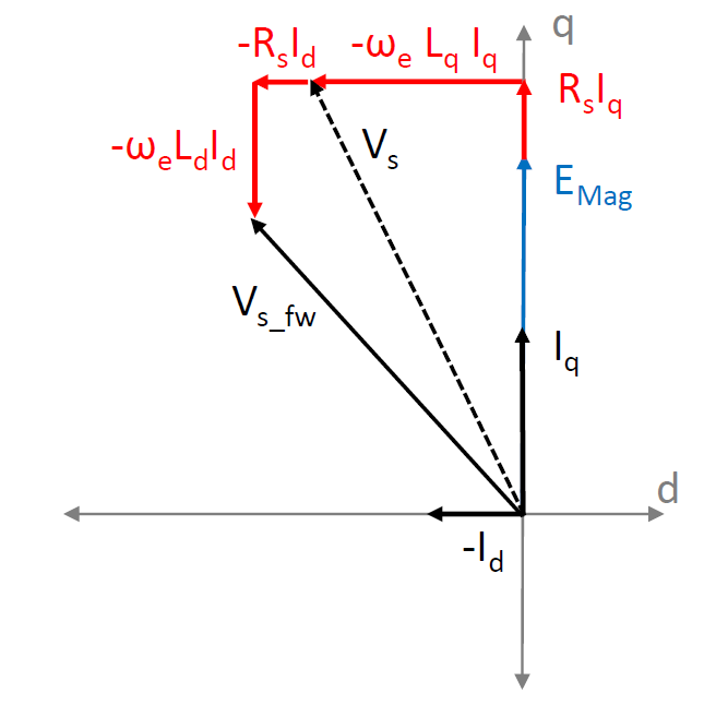
Figure 5.58 PMSM vector diagram: \(I_{d} < 0\)
Since injecting a negative \(I_{d}\) in the motor effectively weakens the air-gap flux, the name flux-weakening (FW) is used. The function of the FW algorithm is the calculation of a suitable reference value for negative \(I_{d}\) to operate the motor at a particular velocity and load.
5.4.1.2. Effect on torque capability
Electromagnetic torque produced in a PMSM with no saliency is given by 5.39. Here, \(P\) is the number of poles in the motor. When \(I_{d} = 0\) (i.e. no flux-weakening), the q-axis current \(I_{q}\) is allowed to increase up to the total rated current of the motor. This results in the rated torque output from the motor.
However, with a negative \(I_{d}\), the maximum allowed value of the q-axis current reduces to limit the total current magnitude of the motor as per 5.40 given below. Here, \(I_{\max}\) is the maximum current amplitude, which is determined by the rated current of the motor or of the drive.
With the reduction in \(I_{q\_limit}\), the torque capability of the motor also reduces. This reduction is more as the motor velocity increases. Figure 5.59 shows normalized plots of torque versus velocity for a non-salient motor. The per unit motor parameters are indicated at the top of the figure. 5.41 is used for calculating the per unit values of motor parameters. Here, \(I_{1}\) is the maximum current and \(V_{1}\) is the nominal back-emf voltage at nominal speed.
The outermost dashed red curve shows the maximum possible torque as a function of velocity. The solid red curves are constant-current plots and the solid black curves are constant-voltage plots. The region shaded light blue is without any FW, while the region shaded pink is the FW region. The dashed curve \(A-D_1-O-A'\) shows the transition between FW and no-FW regions, while the dashed curve \(P-D_2-B-C-P'\) shows the limiting boundary of the FW region. It can be seen that the maximum torque value in the FW region is lower than that in the no-FW region, and it reduces as the velocity increases.
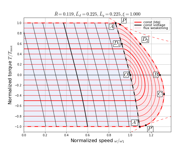
Figure 5.59 Torque-Velocity Plots: Non-salient Motor
For a salient-pole motor, the torque equation is given by 5.42. In this equation, there is an additional reluctance torque term which arises due to motor saliency.
With a negative \(I_{d}\), even though the reluctance torque term gives a positive value, there is a reduction in the first term due to the reduction in \(I_{q\_limit}\). The reduction in the first term dominates over the increase in the second term, thereby reducing the overall torque capability of the motor. The torque-velocity plots for a salient-pole motor are similar to those for a non-salient motor.
5.4.1.3. Flux-weakening algorithms
The flux-weakening algorithm could be implemented in different ways. Some of these methods use an open-loop approach based on motor equations. Other methods implement a closed-loop approach by adding a controller in the FW algorithm. In MCAF R6, an equation-based FW algorithm is implemented. This equation-based algorithm is an open-loop algorithm based on motor equations and does not include an additional controller. Details of this algorithm are given in the section below.