5.4.1.3.1. Equation based flux-weakening
5.4.1.3.1.1. Overview
The flux-weakening (FW) module is required to calculate a suitable d-axis current reference \(I_{d\_fw}\) so as to operate the motor at a velocity higher than the rated velocity without increasing the motor voltage. In MCAF R6, an equation-based algorithm is implemented for flux-weakening. This algorithm is based on an open-loop approach of calculating the current reference for FW operation (\(I_{d\_fw}\)) using the motor voltage equations. Depending on the application requirements, the user can enable or disable flux-weakening.
5.4.1.3.1.2. Flow chart and description
Figure 5.60 shows the flow chart of the flux-weakening algorithm.
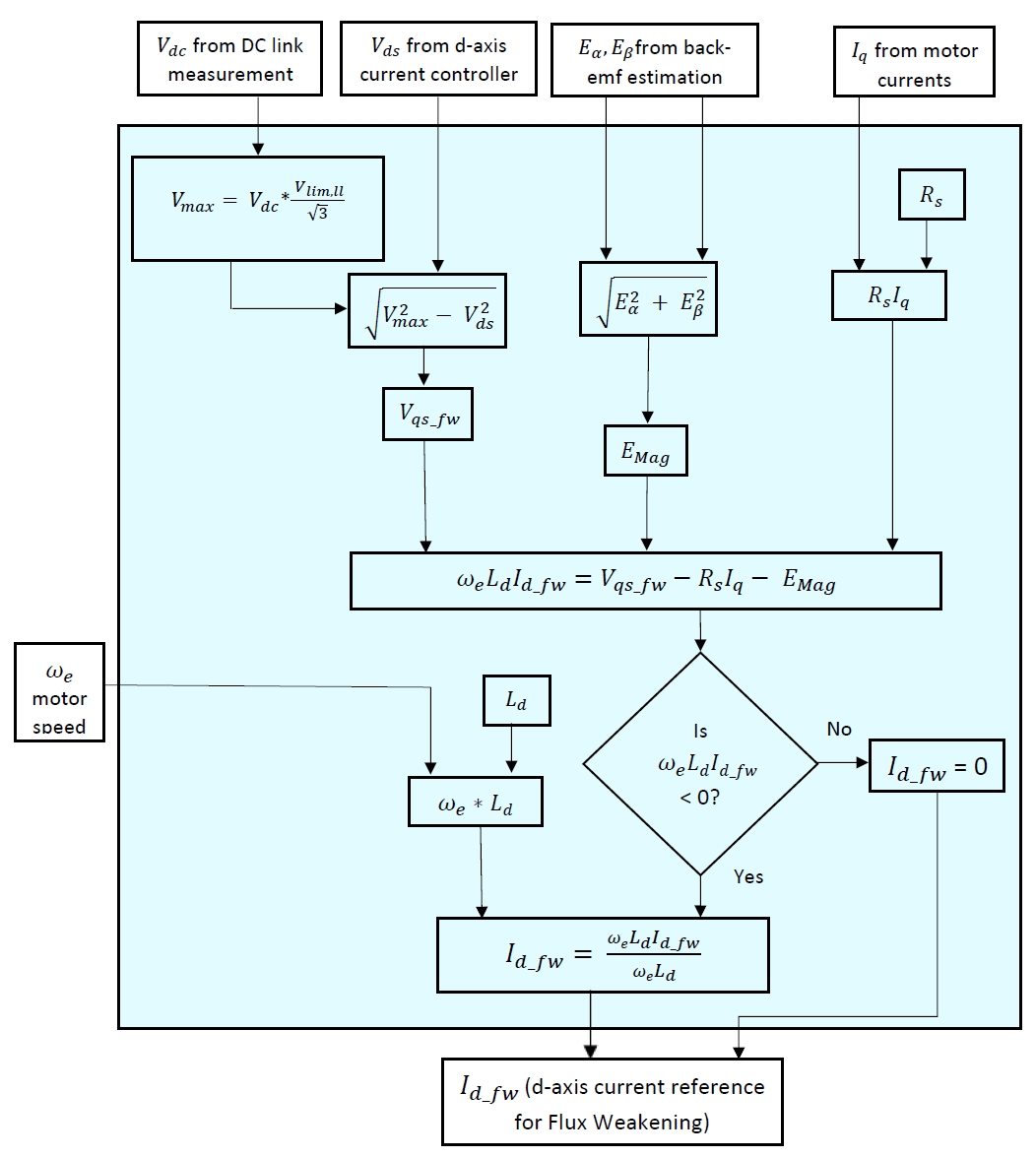
Figure 5.60 Flux-weakening algorithm flow chart
The equation-based FW algorithm performs two important tasks. First, it checks if there is a need for injecting a negative \(I_{d}\) in the motor. This is done by considering the q-axis voltage equation of the motor in the steady state given by 5.43. If the available q-axis voltage (\(V_{qs\_fw}\)) is enough to overcome the addition of \(R_{s}I_{q} + E_{mag}\), there is no need for FW and \(I_{d\_fw}\) is made equal to zero. Here, \(E_{Mag}\) is the back emf magnitude.
The available q-axis voltage (\(V_{qs\_fw}\)) is calculated by taking the d-axis stator voltage (\(V_{ds}\)) as an input and performing the following calculation. Here, \(V_{\max}\) is the maximum possible voltage that can be safely applied to the motor. This is calculated based on the value of DC link voltage \(V_{dc}\) and a voltage limit multiplier \(V_{lim,ll}\) as mentioned in Parameter Customization.
The terms on the right hand side of 5.43 are calculated by adding \(E_{Mag}\) to \(R_{s}I_{q}\). The difference between \(V_{qs\_fw}\) and (\(R_{s}I_{q} + E_{Mag}\)) is then calculated. If this difference is positive, it means that there is sufficient q-axis voltage available to operate at that velocity and load. In this case, \(I_{d\_fw}\) is made equal to zero.
If this difference comes out to be negative, there is a need for flux-weakening and the algorithm then proceeds to calculate the reference current \(I_{d\_fw}\). As seen from 5.43, the calculated difference should match the term \(\omega L_{d} I_{d}\) so as to satisfy this equation. This difference term is divided by \(\omega L_{d}\) to find \(I_{d\_fw}\). After calculation, \(I_{d\_fw}\) is an input to the D-axis current reference generation module, where it is used for \(I_{d\_ref}\) generation.
5.4.1.3.1.3. Implementation notes
Following are some important points related to equation-based FW implementation.
- Filter on \(E_{Mag}\): After calculation, the back emf magnitude \(E_{Mag}\) is passed through a low-pass filter to smooth it out. This filtered value is then used for the calculation of \(I_{d\_fw}\).
- Voltage limit: The maximum voltage magnitude (\(V_{\max}\)) is the limit on the magnitude of voltage. This is also equal to the voltage that is applied to the motor in the flux-weakening region of operation. It is calculated from the DC link voltage magnitude and the voltage limit parameter (\(V_{lim,ll}\)). The calculation is based on the following equation. The \(\sqrt{3}\) in the denominator appears due to the conversion from the line-line voltage to the line-neutral voltage.
5.4.1.3.1.4. Factors affecting flux-weakening operation
Effect of \(V_{\max}\): The value of \(V_{\max}\) plays an essential role in the FW operation. It affects the calculated value of the available q-axis voltage (\(V_{qs\_fw}\)), which in turn affects the velocity at which the motor makes a transition to the FW region of operation. It should be noted that this value is calculated based on the DC link voltage (\(V_{dc}\)) and voltage limit parameter (\(V_{lim,ll}\)). The maximum value of \(V_{lim,ll}\) is 1.
A simplified set of equations is given below to understand the relation between the value of \(V_{\max}\) and the velocity at which a transition is made to the FW region. 5.46 gives steady-state motor voltage equations along with the calculation of the available q-axis voltage (\(V_{qs\_fw}\)).
(5.46)\[\begin{aligned} V_{ds} &= - \omega L_q I_q \\ V_{qs\_fw} &= \sqrt{V_{\max}{}^2 - V_{ds}{}^2} \\ V_{qs\_fw} &= R_s I_q + \omega L_{d} I_{d} + E_{Mag}\\ E_{Mag} &= \omega_e \Psi_{PM} \end{aligned}\]As the motor velocity (considered to be positive here) increases, magnitude of \(V_{ds}\) increases and as a result, the magnitude of \(V_{qs\_fw}\) reduces. Due to this, the initially positive term \(\omega L_{d} I_{d}\) as calculated from \(V_{qs\_fw}\) equation reduces in magnitude. At the boundary of transition to the FW region, this term becomes zero. If the stator resistance term (\(R_{s} I_{q}\)) is neglected for simplification, the velocity at which the transition happens to the FW region (\(\omega_{fw\_tr}\)) can be given by 5.47. Thus, as \(V_{\max}\) increases, \(\omega_{fw\_tr}\) increases.
(5.47)\[\omega_{fw\_tr} = \frac{V_{\max}}{\sqrt{(L_q I_q)^2 + \Psi_{PM}{}^2}}\]For a given \(V_{lim,ll}\), if the DC link voltage is higher, \(V_{\max}\) will also increase in proportion (5.45). This will result in the motor making a transition to the FW region at a higher velocity. Likewise, reduction in the value of DC link voltage or the value of \(V_{lim,ll}\) will cause the transition to the FW region to happen at a lower velocity.
Velocity extension in FW region: The limit on velocity extension in the FW region depends on factors such as motor’s rated current, inductance and back emf constant. 5.48 shows the relation between the approximate gain in velocity as a function of motor maximum current \(I_{\max}\), \(L_{d}\) and \(\Psi_{PM}\). For motors with larger inductance and larger rated current, the velocity extension in FW region is more, while for motors with lower back emf constant, the extension in the FW region is found to be more.
(5.48)\[\frac{\omega_{\max}}{\omega_{rated}} = \frac{1}{1 - \frac{L_d I_{\max}}{\Psi_{PM}}}\]Figure 5.61 shows the torque-velocity capability curves for a non-salient motor. The per unit motor parameters are indicated at the top of the figure. The outermost dashed red curve shows the maximum possible torque as a function of velocity. The solid red curves are constant-current plots and the solid black plots are constant-voltage plots. The region shaded light blue is without any FW, while the region shaded pink is the FW region. The shaded curve \(A-D_1-O-A'\) shows the boundary between FW and no-FW regions, while the shaded curve \(P-D_2-B-C-P'\) shows the limiting boundary of the FW region. Point B and point C show the velocity at no-load condition in the FW motoring and FW generating regions, respectively. These values are the theoretical maximum achievable velocity values in absence of Coulomb friction and viscous drag. In Figure 5.61, the maximum velocity in motoring region is around 1.28 per unit.
Figure 5.62 shows the torque-velocity capability curves for the same motor, however with a 50% increase in motor inductance values. It can be seen that the velocity limit in the FW motoring region is increased and is around 1.5 per unit.
Figure 5.63 shows the torque-velocity capability curves for the same motor with original inductance values, however with a 50% increase in motor current rating. The velocity limit in the FW motoring region is around 1.48 per unit and is larger as compared to the value of 1.28 per unit in Figure 5.61.
Figure 5.64 shows the torque-velocity capability curves for the same motor with original inductance values and motor current rating, however with a back emf constant reduced to 75% of its original value. The velocity limit in the FW motoring region is around 1.4 per unit and is larger as compared to the value of 1.28 per unit in Figure 5.61.
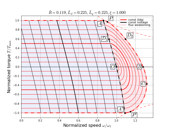
Figure 5.61 Torque-velocity capability curves for a non-salient motor
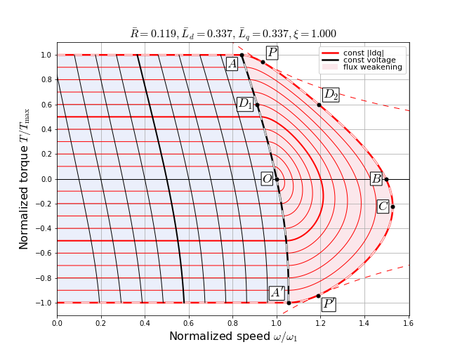
Figure 5.62 Torque-velocity capability curves for a non-salient motor, with higher inductance
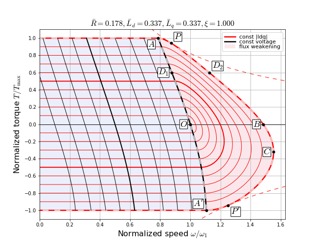
Figure 5.63 Torque-velocity capability curves for a non-salient motor, with higher current rating
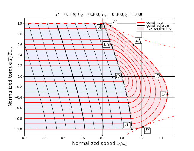
Figure 5.64 Torque-velocity capability curves for a non-salient motor, with lower back emf constant