5.3.3. Angle-tracking Phase-locked Loop (ATPLL)

5.3.3.1. Overview

The Angle-tracking Phase-locked Loop (ATPLL) is a velocity and rotor angle estimation algorithm provided for sensorless closed-loop velocity control of a PMSM. The algorithm has a PLL-like structure, and it estimates the correct rotor velocity and angle by making the d-axis component of the back emf equal to zero in steady state. The rotor velocity and angle errors are eliminated in steady state due to a PI controller module included in the structure of the ATPLL estimator. The ATPLL estimator algorithm can be used for the estimation of rotor velocity and rotor angle for PMSM motors with or without rotor saliency.

5.3.3.2. Implementation Block Diagram and Description

Figure 5.51 shows the basic principle of the ATPLL estimator. Here, The outputs of the estimator are estimated rotor velocity (\(\hat\omega\)) and estimated rotor angle (\(\hat\theta\)). The d-axis component (\(E_d\)) of the back-emf is calculated from the motor stator voltages (\(V_{\alpha}\), \(V_{\beta}\)) and stator currents (\(I_{\alpha}\), \(I_{\beta}\)). The reference value of \(E_d\) is zero, therefore the error becomes equal to \(- E_d\). This error is fed to a PI controller. The output of the PI controller is added with a feedforward velocity term \(\omega_{ref}\), and this addition is the estimated velocity \(\hat\omega\). The estimated velocity is integrated to obtain the estimated rotor angle \(\hat\theta\).

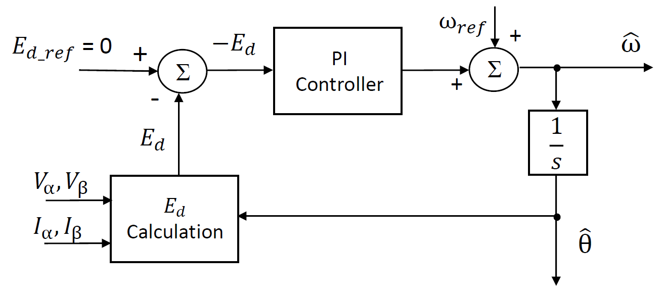
Figure 5.51 ATPLL: Generic Block Diagram

The MCAF implementation of the ATPLL estimator is shown in Figure 5.52. A brief description of the different blocks used in the ATPLL structure is given below.

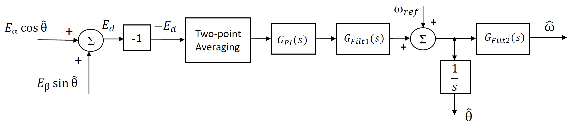
Figure 5.52 ATPLL implementation

• Inputs: The ATPLL algorithm begins by calculating the back-emf components \(E_{\alpha}\) and \(E_{\beta}\) from the stator voltages (\(V_{\alpha}\), \(V_{\beta}\)) and stator currents (\(I_{\alpha}\), \(I_{\beta}\)) using the motor resistance and inductance values. These back-emf values are then used for further calculation of \(- E_d\) as shown in Figure 5.52. For calculation of \(E_{\alpha}\) and \(E_{\beta}\), equation 5.27 is used for motors without significant rotor saliency, and equation 5.28 is used for motors with rotor saliency. Motors are categorised into those with and without significant rotor saliency based on their Saliency Constant. In 5.27, \(R_{s}\) and \(L_{s}\) are per-phase stator winding resistance and inductance values respectively. In 5.28, \(\theta\) is the rotor angle and \(L_0\) and \(L_1\) are given by 5.29.

(5.27)\[\begin{bmatrix} E_{\alpha} \\ E_{\beta} \end{bmatrix} = \begin{bmatrix} V_{\alpha} \\ V_{\beta} \end{bmatrix} - \begin{bmatrix} R_{s} & 0 \\ 0 & R_{s} \end{bmatrix} \begin{bmatrix} I_{\alpha} \\ I_{\beta} \end{bmatrix} - \begin{bmatrix} L_{s} & 0 \\ 0 & L_{s} \end{bmatrix} \frac{d}{dt}\begin{bmatrix} I_{\alpha} \\ I_{\beta} \end{bmatrix}\]

(5.28)\[\begin{bmatrix} E_{\alpha} \\ E_{\beta} \end{bmatrix} = \begin{bmatrix} V_{\alpha} \\ V_{\beta} \end{bmatrix} - \begin{bmatrix} R_{s} & 0 \\ 0 & R_{s} \end{bmatrix} \begin{bmatrix} I_{\alpha} \\ I_{\beta} \end{bmatrix} - \frac{d}{dt}\begin{bmatrix}\begin{bmatrix} L_{0}+L_{1}\cos 2\theta & L_{1}\sin 2\theta \\ L_{1}\sin 2\theta & L_{0}-L_{1}\cos 2\theta \end{bmatrix} \begin{bmatrix} I_{\alpha} \\ I_{\beta} \end{bmatrix} \end{bmatrix}\]

(5.29)\[L_0 = \frac{L_d + L_q}{2}, L_1 = \frac{L_d - L_q}{2}\]

• Two-point Averaging: As mentioned above, first \(- E_d\) is calculated from \(E_{\alpha}\) and \(E_{\beta}\) and is fed to the Two-point Averaging block. This block helps to smooth the input to the Proportional-Integral (PI) controller (\(G_{PI}(s)\)).
• \(G_{PI}(s)\) : This block represents a PI controller which is the backbone of the ATPLL estimator. In steady state, the input to the PI controller (which is: \(- E_d\)) is reduced to zero, thereby reducing the steady-state error in the estimated velocity and angle to zero as well. The s-domain representation of \(G_{PI}(s)\) is as given below:

(5.30)\[G_{PI}(s) = K_p + \frac{K_i}{s} \]

• \(G_{Filt1}(s)\) : This is a low-pass filter at the output of the PI controller. After filtering, the output is added to the reference velocity (\(\omega_{ref}\)). The result of this addition is the unfiltered estimated velocity and is integrated to calculate the estimated rotor angle (\(\hat\theta\)). The s-domain representation of \(G_{Filt1}(s)\) is as given below, where, \(\tau_1\) is the filter time constant.

(5.31)\[G_{Filt1}(s) = \frac{1}{\tau_1 s + 1} \]

• \(G_{Filt2}(s)\) : The result of the addition of the PI controller output and the reference velocity is further filtered using this low-pass filter. The output of this filter is the estimated rotor velocity (\(\hat\omega\)). The s-domain representation of \(G_{Filt2}(s)\) is as given below, where, \(\tau_2\) is the filter time constant.

(5.32)\[G_{Filt2}(s) = \frac{1}{\tau_2 s + 1} \]

Following are some important points related to the PI controller and low-pass filter blocks.

• To obtain a stable dynamic performance of the ATPLL estimator over the entire operating velocity range, the integral gain \(K_i\) is made dependent on the reference velocity \(\omega_{ref}\). To support motors with different parameter values, the proportional and integral gains \(K_p\) and \(K_i\) are made dependent on the motor’s back-emf constant \(K_e\). Empirical tuning of the PI controller gains simplifies the design significantly. The empirical equations for \(K_p\) and \(K_i\) are given in equation 5.33.

(5.33)\[\begin{aligned} K_{p} &= \frac{1.9}{K_e} \cr K_{i} &= \frac{\omega_{ref}}{30 K_e} \end{aligned}\]

• Reversal of velocity is supported by the ATPLL estimator. In order to make this possible, the signs of PI controller gains are reversed based on the sign of the reference velocity.
• Filter constants \(\tau_1\) and \(\tau_2\) are decided based on the performance of the control algorithm for a range of motors. The filter constants are fixed in MCAF R5, but may be made adjustable in a future revision.

5.3.3.3. Application to PMSMs with Saliency

In case of interior permanent-magnet motors (IPMSMs), the \(d\)- and \(q\)-axis inductances are not equal; typically \(L_q\) is larger than \(L_d\). In order to quantify the degree of saliency in the rotor, the following saliency constant is defined. Here, \(\xi\) is equal to \(\frac{L_q}{L_d}\).

(5.34)\[\text{Saliency Constant} = 1 - \frac{1}{\xi} \]

It can be noted that the saliency constant is equal to 0 for motors with no saliency and increases toward 1 as the saliency increases. For a correct rotor velocity and angle estimation, it is important that the relevant equations are used by the estimator, which are different for motors with salient and non-salient rotors. In order to differentiate the salient motors from the non-salient ones, a saliency constant threshold of 0.25 is defined. Thus, the motors satisfying the following condition are considered to be salient pole motors.

(5.35)\[1 - \frac{1}{\xi} > 0.25 \]

This can further be simplified to

(5.36)\[\xi > \frac{4}{3}. \]

The ATPLL estimator accommodates motors both with salient and non-salient rotors by a suitable choice of equations in its algorithm, thus preserving the accuracy of rotor velocity and angle estimation.

5.3.3.4. Sample Results

The following results are obtained from numerical simulation for a Leadshine 400 motor. A superimposed plot of actual rotor velocity and the estimated rotor velocity by the ATPLL estimator is shown in Figure 5.53 along with the plot showing the error in estimated velocity. It can be observed that the steady-state velocity error is zero.

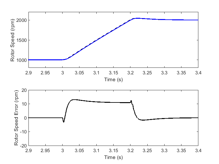
Figure 5.53 Estimated Rotor Velocity by the ATPLL

A superimposed plot of actual rotor angle and the estimated rotor angle by ATPLL estimator along with the error in the estimated angle is shown in Figure 5.54. This plot is for the same velocity transient shown in Figure 5.53. It can be seen that the steady-state angle error is zero.

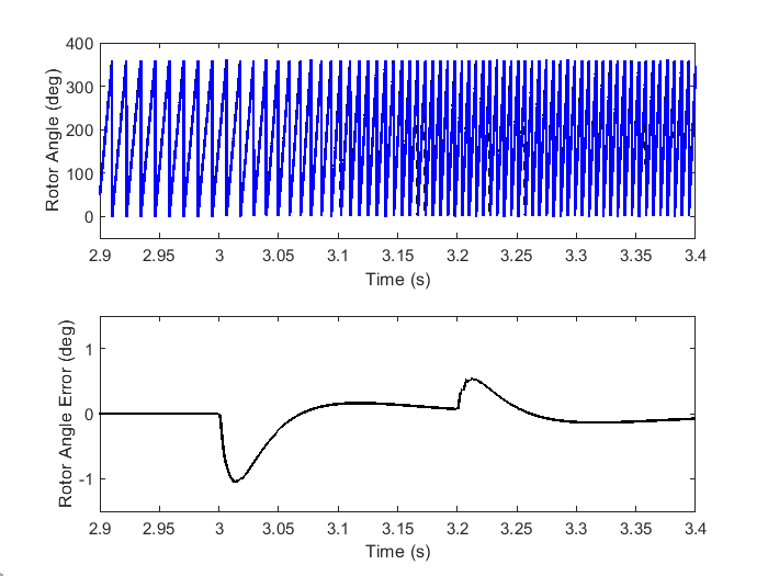
Figure 5.54 Estimated Rotor Angle by the ATPLL