5.6.5.1. Simple dynamic current limit
This algorithm approximates a differential equation for a current \(I_x\), and determines the current limit \(I_{\lim}\) as the minimum of \(I_x\) and a predetermined fixed peak current \(I_{\rm peak}\). This equation is given below:
The current relaxes asymptotically to a “horizon” current \(I_{\rm horz}\). An illustrated example is shown in Figure 5.90, with \(I_{\rm horz} =\) 60 A, \(I_{\rm peak} =\) 30 A, \(I_{\rm cont} =\) 10 A, \(\tau =\) 6 seconds.
The horizon current also determines the slew rate of current as it rises from the continuous current level; specifically, if current command changes in a step from \(I_{\rm cont}\) to zero, the slew rate of the current limit is \((I_{\rm horz}-I_{\rm cont})/\tau\). In Figure 5.90, this occurs at \(t=\) 3 seconds.
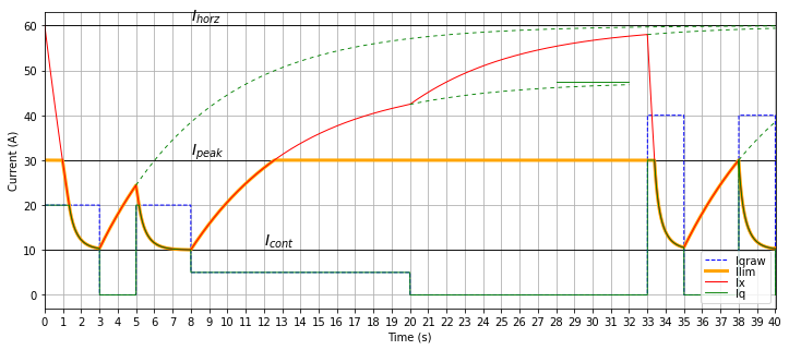
Figure 5.90 Simulation of simple dynamic current limit. Only q-axis current \(I_q\) is shown; the d-axis current \(I_d\) is assumed to be regulated to zero or very near zero.
In this case, if the motor current has been low enough for a long enough time that the current \(I_x\) relaxes back nearly to the horizon current, the drive can provide 20 A current for about 1.3 seconds, decreasing to the continuous limit of 10 A after about 3 seconds. Operation at the full peak current of 30 A will use up the transient capacity more quickly, lasting for about 0.4 seconds, decreasing to the continuous limit of 10A after about 2 seconds.
The motor torque can be fairly substantial and still allow the current limit to return to near-maximum values, because the thermally-limited components heat up proportionally to the square of the current. Even 50% of the continuous current limit causes only 25% of the temperature rise of the continuous current, which allows the motor and transistors to cool down. This is shown in Figure 5.90 after \(t=\) 8 seconds. (Conversely, twice the continuous current limit produces four times the power dissipation.)
Note that since \(I_d{}^2 + I_q{}^2\) accumulates to reduce the current limit, neither the direction of current nor the direction of rotation matter; positive and negative values of \(I_q\) affect the current limit equally.
5.6.5.1.1. Choice of parameters
The choice of parameters here will be different for each board and should be validated to ensure motor and transistor are kept in their safe operating region.
Aside from peak and continuous limits, which are covered in the main section on dynamic current algorithms, the other two parameters should be selected empirically:
time constant \(\tau\) should have some similarity to the thermal dynamics of the real system. Choosing too small of a value will lower the current limit prematurely, so if the motor and transistor have not heated up very much, then a larger time constant should be used. Similarly, if the motor or transistor have heated up to an unsafe level before the current limit decreases, then the time constant is probably too large.
horizon current \(I_{\rm horz}\) impacts how much thermal headroom is present: larger values will allow the current limit to stay higher for a longer period of time, and will allow the current limit to increase more quickly once the motor current drops back to a small value.
5.6.5.1.2. Implementation notes
Since the thermal dynamics are fairly slow (tenths of seconds to tens of seconds), this algorithm is partitioned, with most of this algorithm executes at a decimated rate, compared to the current control sample rate.
At the full sample rate (sample time \(T_s\)), the squared amplitude of current \(I_d{}^2 + I_q{}^2\) is accumulated.
The rest of the dynamic current limit algorithm runs at a decimated rate (period = \(nT_s\) with \(n=128\) by default) that updates the current \(I_x\) based on the accumulated squared current.